Spoken term Discovery / Word segmentation
Contents
Task & Goal
Just as the infant learns the words of their language by listening, spoken term discovery seeks to find recurring patterns in the input, proposing a set of boundaries delimiting the start and end of proposed word tokens discovered in the speech, and category labels indicating proposed word types1.
This problem was explored by several papers prior to the ZRC ( Citation: 2008 Park, A. & Glass, J. (2008). Unsupervised Pattern Discovery in Speech. IEEE Transactions on Audio, Speech, and Language Processing, 16(1). 186–197. ; Citation: 2010 Zhang, Y. & Glass, J. (2010). Towards multi-speaker unsupervised speech pattern discovery. ; Citation: 2011 Jansen, A. & Van Durme, B. (2011). Efficient spoken term discovery using randomized algorithms. IEEE. ; Citation: 2012 Muscariello, A., Gravier, G. & Bimbot, F. (2012). Unsupervised Motif Acquisition in Speech via Seeded Discovery and Template Matching Combination. IEEE Transactions on Audio, Speech and Language Processing, 20(7). 2031–2044. ; Citation: 2013 Jansen, A., Thomas, S. & Hermansky, H. (2013). Weak top-down constraints for unsupervised acoustic model training. IEEE. ) , and served as inspiration for the challenge itself. Although the task of “finding words” seems intuitively simple, it is made up of at least three sub-problems which we evaluate separately (see Figure 1).
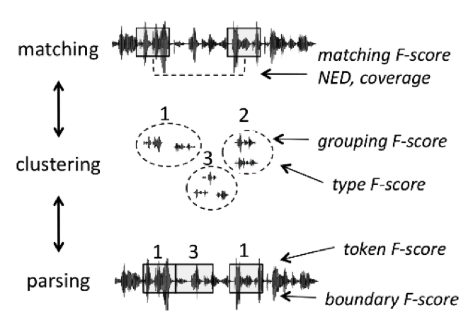
Figure 1. Term discovery subtasks and metrics
-
The matching sub-problem is to find all pairs of speech fragments that are instances of the same sequence of phonemes. This can be evaluated based on how phonemically similar the discovered fragments are using the gold transcription (normalized edit distance: NED) and how much of the corpus they cover (coverage).
-
The lexicon discovery sub-problem is to group these fragments into clusters (as opposed to simple pairwise matching). The goal is to find a lexicon of types. A proposed cluster can be evaluated based on how well the members match on the sequence of phonemes (Grouping) and how well the sets match the gold-standard lexicon of word types (Type F-score).
-
The word segmentation sub-problem attempts to find onsets and offsets of fragments that are aligned with the word boundaries as defined in the gold-standard text: we use the token and boundary F-scores as is usual in text-based word segmentation.
To maximize comparability with text-based word discovery approaches, all of these evaluations are done at the level of the phonemes obtained forced aligning the test set with its phoneme transcription. Any discovered speech fragment is converted into its transcription, including potentially stranding phonemes on the left or right edge if it contains more than 30 ms of that phoneme or more than 50% of its duration.
Metrics
Notations
All of our metric assume a time aligned transcription, where $T_{i,j}$ is the (phoneme) transcription corresponding to the speech fragment designed by the pair of indices $\langle i,j \rangle$ (i.e., the speech fragment between frame $i$ and $j$ ). If the left or right edge of the fragment contains part of a phoneme, that phoneme is included in the transcription if is corresponds to more than more than 30ms or more than 50% of it’s duration.
We first define the set related to the output of the discovery algorithm:
- $C_{disc}$: the set of discovered clusters (a cluster being a set of fragments with the same category name).
From these, we can derive:
-
$F_{disc}$: the set of discovered fragments, $F_{disc} = { f | f \in c , c \in C_{disc} }$
-
$P_{disc}$: the set of non overlapping discovered pairs, $P_{disc} = { {a,b} | a \in c, b \in c, \neg \textrm{overlap}(a,b), c \in C_{disc} }$
-
$P_{disc^*}$: the set of pairwise substring completion of $P_{disc}$, which mean that we compute all of the possible minimal path realignments of the two strings, and extract all of the substrings pairs along the path (e.g., for fragment pair $\langle abcd, efg \rangle$: $\langle abc, efg \rangle$, $\langle ab,ef \rangle$, $\langle bc, fg \rangle$, $\langle bcd, efg \rangle$, etc).
-
$B_{disc}$: the set of discovered fragment boundaries (boundaries are defined in terms of $i$, the index of the nearest phoneme boundary in the transcription if it is less than 30ms away, and -1 (wrong boundary) otherwise)
Note:
Two fragments a and b overlap if they share more than half of their temporal extension.
Next, we define the gold sets:
-
$F_{all}$: the set of all possible fragments of size between 3 and 20 phonemes in the corpus.
-
$P_{all}$: the set of all possible non overlapping matching fragment pairs. $P_{all}={ {a,b }\in F_{all} \times F_{all} | T_{a} = T_{b}, \neg \textrm{overlap}(a,b)}$.
-
$F_{goldLex}$: the set of fragments corresponding to the corpus transcribed at the word level (gold transcription).
-
$P_{goldLex}$: the set of matching fragments pairs from the $F_{goldLex}$.
-
$B_{gold}$: the set of boundaries in the parsed corpus.
Most of our measures are defined in terms of Precision, Recall and F-score. Precision is the probability that an element in a discovered set of entities belongs to the gold set, and Recall the probability that a gold entity belongs to the discovered set. The F-score is the harmonic mean between Precision and Recall.
$$Precision_{disc,gold} = \frac{| disc \cap gold |}{| disc |}$$
$$Recall_{disc,gold} = \frac{| disc \cap gold |}{| gold |}$$
$$F-Score_{disc,gold} = \frac{2}{(1/Precision_{disc,gold} + 1/Recall_{disc,gold})}$$
Matching scores
The evaluation of spoken term discovery systems as matching systems consists of two scores, NED and coverage.
NED, is the average, over all matched pairs, of the Levenshtein distance between their phonemic transcriptions, divided by the max of their phonemic length. It is equal to zero when a pair of fragments have exactly the same transcription, and 1 when they differ in all phonemes.
coverage is the fraction of the discoverable part of the corpus that is covered by all the discovered fragments. The discoverable part of the corpus is found by computing the union of all of the intervals corresponding to all of the pairs of ngrams (with n between 3 and 20). This is almost all of the corpus, except for unigram and bigram hapaxes.
$$ \textrm{NED} = \sum_{\langle x, y\rangle \in P_{disc}} \frac{\textrm{ned}(x, y)}{|P_{disc}|} $$ $$ \textrm{Coverage} = \frac{|\textrm{cover}(P_{disc})|}{|\textrm{cover}(P_{all})|} $$
where
$$ \textrm{ned}(\langle i, j \rangle, \langle k, l \rangle) = \frac{\textrm{Levenshtein}(T_{i,j}, T_{k,l})}{\textrm{max}(j-i+1,k-l+1)} $$ $$ \textrm{cover}(P) = \bigcup_{\langle i, j \rangle \in \textrm{flat}(P)}[i, j] $$ $$ \textrm{flat}(P) = {p|\exists q:{p,q}\in P} $$
Note: the 2015 Benchmark used to have another matching metrics (Matching precision, recall and F-score) comparing $X=P_{disc^* }$ the set of discovered pairs (with substring completion) to $Y=P_{all}$ the set of all possible gold pairs. The precision and recall was computed over each type of pairs, and averaged after reweighting by the frequency of the pair. This method was very expensive computationally, and did not max at 1 if the discovered pairs were small. It was subsequently deprecated.
Clustering scores
Six scores are used to evaluate the performance of a spoken term discovery system in terms of lexicon discovery.
The first three are Grouping Precision, Recall and F-score. These are defined in terms of $P_{clus}$ , the set of all pairs of fragments that are groups in the same cluster, and $P_{goldclus}$ , the set of all non-overlapping pairs of fragments which are both discovered by the system (not necessarily in the same cluster) and have exactly the same gold transcription.
$$ \mbox{Prec:} \sum_{t \in \text { types }\left(P_{\text {clus }}\right)} w\left(t, P_{\text {clus }}\right) \frac{\left|\operatorname{occ}\left(t, P_{\text {clus }} \cap P_{\text {goldclus }}\right)\right|}{\left|\operatorname{occ}\left(t, P_{\text {clus }}\right)\right|} $$
$$ \mbox{Rec:} \sum_{t \in \operatorname{types}\left(P_{\text {goldclus }}\right)} w\left(t, P_{\text {goldclus }}\right) \frac{\left|\operatorname{occ}\left(t, P_{\text {clus }} \cap P_{\text {goldclus }}\right)\right|}{\left|\operatorname{occ}\left(t, P_{\text {goldclus }}\right)\right|} $$
where
$$ P_{clus} = { \langle \langle i, j\rangle , \langle k, l \rangle\rangle | \exists c\in C_{disc},\langle i, j\rangle\in c \wedge \langle k, l\rangle\in c } $$ $$ P_{goldclus} = { \langle \langle i, j\rangle , \langle k, l \rangle\rangle | \exists c_1,c_2\in C_{disc}:\langle i, j\rangle\in c_1 \wedge \langle k, l\rangle\in c_2 \wedge T_{i,j}=T_{k,l} \wedge [i,j] \cap [k,l] = \varnothing } $$
and where t ranges over the types of fragments (defined by the transcription) in a cluster $C$, and $occ(t, C)$ is the number of occurrences of that type, $w$ the number of occurrences divided by the size of the cluster. In other words, Prec is a weighted measure of cluster purity and Rec, of the inverse of the cluster’s fragmentation.
The other three scores are Type Precision, Recall, and F-score. Type precision is the probability that discovered types belong to the gold set of types (real words), whereas type recall is the probability that gold types are discovered. This is a much more demanding. Indeed, a system could have very pure clusters, but could systematically missegment words. Since a discovered cluster could have several transcriptions, we use all of them (rather than using some kind of centroid). We restrict both sets to words between three and twenty segments long.
$$ \textrm{Type precision} = \frac{|\textrm{types}(F_{disc}) \cap \textrm{types}(F_{goldLex})|} {|\textrm{types}(F_{disc})|} $$ $$ \textrm{Type recall} = \frac{|\textrm{types}(F_{disc}) \cap \textrm{types}(F_{goldLex})|} {|\textrm{types}(F_{goldLex})|} $$
Segmentation scores
Parsing quality is evaluated using two sets of 3 metrics. The first set (Token Precision, Recall and F-score) evaluates how many of the word tokens were correctly segmented ($X = F_{disc}$, $Y = F_{goldLex}$). The second one (Boundary Precision, Recall and F-score) evaluates how many of the gold word boundaries were found ($X = B_{disc}$, $Y = B_{gold}$). These two metrics are typically correlated, but researchers typically use the first. We provide Boundary metrics for completeness, and also to enable system diagnostic.
$$ \textrm{Token precision} = \frac{|F_{disc}\cap F_{goldLex}|}{|F_{disc}|} $$ $$ \textrm{Token recall} = \frac{|F_{disc}\cap F_{goldLex}|}{|F_{goldLex}|} $$ $$ \textrm{Boundary precision} = \frac{|B_{disc}\cap B_{gold}|}{|B_{disc}|} $$ $$ \textrm{Boundary recall} = \frac{|B_{disc}\cap B_{gold}|}{|B_{gold}|} $$
The details of these metrics are given in Ludusan et al (2014) ( Citation: Ludusan, Versteegh & al., 2014 Ludusan, B., Versteegh, M., Jansen, A., Gravier, G., Cao, X., Johnson, M. & Dupoux, E. (2014). Bridging the gap between speech technology and natural language processing: An evaluation toolbox for term discovery systems. ) . The only divergence between this paper and the present measures, is that contrary to the paper, we compute these scores on the entirety of the corpus, rather than on the covered corpus. It is necessary to do this if we want to compare systems that will cover different subsets of the corpus. In the implementation for the challenge, we use a subsampling scheme whereby the corpus is cut into 10 equal parts and each metric is computed on each of the subsample separately and then averaged. This enables the computation to be more tractable (especially for the matching metric which requires substring completion), and also to provide a standard deviation measure for each metric. We also provide, in addition to each metric ran on the entire corpus, the same metric restricted to within talker matches. This is to enable the evaluation of systems that are specialized in within talker spoken term discovery.
Comparison with other metrics
Contrary to ABX, the metrics computed here assume that the models explicitely compute patching pairs, cluster IDs and segment boundaries. Yet, it is possible that a system could discover words in an implicit fashion, making these evaluations impossible to run. Implicit or zero shot metrics are possible and may be added in subsequent evolutions of ZRC.
Bibliography
$^*$The full bibliography can be found here
- Jansen, Thomas & Hermansky (2013)
- Jansen, A., Thomas, S. & Hermansky, H. (2013). Weak top-down constraints for unsupervised acoustic model training. IEEE.
- Jansen & Van Durme (2011)
- Jansen, A. & Van Durme, B. (2011). Efficient spoken term discovery using randomized algorithms. IEEE.
- Ludusan, Versteegh, Jansen, Gravier, Cao, Johnson & Dupoux (2014)
- Ludusan, B., Versteegh, M., Jansen, A., Gravier, G., Cao, X., Johnson, M. & Dupoux, E. (2014). Bridging the gap between speech technology and natural language processing: An evaluation toolbox for term discovery systems.
- Muscariello, Gravier & Bimbot (2012)
- Muscariello, A., Gravier, G. & Bimbot, F. (2012). Unsupervised Motif Acquisition in Speech via Seeded Discovery and Template Matching Combination. IEEE Transactions on Audio, Speech and Language Processing, 20(7). 2031–2044.
- Park & Glass (2008)
- Park, A. & Glass, J. (2008). Unsupervised Pattern Discovery in Speech. IEEE Transactions on Audio, Speech, and Language Processing, 16(1). 186–197.
- Zhang & Glass (2010)
- Zhang, Y. & Glass, J. (2010). Towards multi-speaker unsupervised speech pattern discovery.
-
Note here, that contrary to Task 1, we ask systems to explicitly return linguistically interpretable representations (boundaries and cluster labels) instead of a representation that simply satisfies certain functional properties. ↩︎